Abstract : The simulation of
trapped particles is carried out. It is one of the
numerous factors for the
optimisation of magnetic fields and coils. In the medium term the objective
is to have several codes or expressions to design a sound set of coils for
UST_1 . The described experience simulates 40 particles and generates 6
trapped particles.
General description
Trapped particles are important in
stellarators, they are even more relevant than in tokamaks. As an evolution of the
SimPIMF v1.0 code, the simulation of trapped particles seemed an interesting
posibility.
The new addition to the code [1] , that evolves to the version SimPIMF v1.1 is the expression of the effective force against one particle in a variable magnetic field. Only the component parallel to B is considered.
The projection of F = - μm Grad B [2] on B gives an acceleration which is applied on each step of the simulation.
Additionally the principle of energy conservation is fulfilled to obtain the new radial velocity of the particle.
It is not known if this procedure is totally correct, but if the magnetic moment remains constant and the simulations agree with the real experiments the symptoms will be positive.
Modelling
The model of the simulations is described in
[3]. It is a classical stellarator with l=2 m=6 that have similar
dimension and shape as CTH, a torsatron in Auburn University. The model can
be seen in Graph 1. CTH is a l=2 m=5
torsatron and here it is l=6 because this model is an older and rough model.
Besides,
at the moment, stellarators seem a better option than torsatrons. The geometrical major radius is 0.75m.
The simulation in Graph 2 has the next parameters:
Steps = 600000
Time per step = 0.1 NanoSeconds
Number of particles = 40 , 20 e- and 20 H+
Reference temperature = 100000 K . See note (1)
Volume of particle breeding : Cylindrical ring of Z =0.16m , major central radius 0.68m, width of the ring = 0.16m
Procesing time = 8553 , aprox 2 hours and a half.
The velocity drift due to the electric field is switch off.
(1)
A maxwellian distribution is not created yet. In this
case a uniform distribution of energy is used, from 0.25 * T up to 5/4 * T,
all with the same probability. The particles have energy in the interval 10
-19 J, 10-18 J
Results
Several runs are carried out for both models. Only two are
described.
Model A : Gradient in X . At the begining a simple gradient of magnetic field in the X coordinate were modelled to test the general behaviour of the expresions. The energy is conserved, the particle bounces repetedly and simetrically, and aboveall the magnetic moment is well conserved which is a consecuence of the system because it is not included explicity in the code.
Model B : The model is described above and in [3]. The confinement of this model may be poor because it was created without any rule of good plasma confinement. So this simulation could be additionally useful to know what is a deficient confinement or system of coils.
In Graph 2 the plan view from the simulation is shown. Each colour is one of the 20 first particles. The rest are not recorded in this case. The lines that go to the centre help to see and catch each particular particle.
One part of the results file is the number of bounces of each particle, as shown partially here:
Order number Number of bounces
0 53
1 0
2 4
3 0
4 0
- - - - -
16 15
18 4
- - - - -
The trajectories of 3 trapped particles is shown in Graph 3. One is
a helically trapped particle and two are toroidally trapped.
Six particles out of 40 were trapped with the conditions described above.
A detail of a poloidal view of the helically trapped particle, number 0, appears in Graph 4. The graphical representation is reduced in number of points when the nº of steps is high. Periodically some areas are displayed with higher resolution. The yellow bunches are these areas and the rotation of the particle is seen though with difficult because this is a 600KSteps simulation.
The velocity drift is due to the gradient of B and the centrifugal force. The part of the code referent to the electrical field is switch off so it do not produce drift
The effect of this downwards drift appears in the Graph 4. If the electrical field were in the model an outwards drift will be added.
Coments
The simulation of up to 1000 particles should be possible using a PC and 24 hours by making only minor improvements on the computation speed. The elimination of the Larmour rotation will speed the code far more.
A deviation of the trajectories of some trapped particles when decreasing the "Step" length has been observed. This deviation is minimum in SimPIMF v1.0 so it needs to be analysed and compared.
The reason for the difference between
the typical graphical representations of banana orbits and helically trapped
particles, [4] Figure 10, and the ones here is not clear. Perhaps in the
graphical representations the wide of the "banana" is expanded for
representation reasons.
Further developments
The code should be tested
against other recognised codes and data from real experiments. The
compensating effects of toroidally and hellically trapped particles should
be undertood, [4] page7. Test the code against deviations due to "Step"
lenght. Use the application as a component of the optimisation of coils
References
[1] "Development of a basic code for Monte Carlo simulation of trajectories of plasma particles", Vicente M. Queral . See “List of all past R&D" in this web.
[2] "Fusion research" T.J. Dolan, Pergamon Press. Pg 154
[3] "Simulation of magnetic surfaces in a classical stellarator using SimPIMF v1.0", Vicente M. Queral . See “List of all past R&D" in this web.
[4] "STELLARATORS" , D.A. Hartmann, Max-Planck Institut für Plasmaphysik.
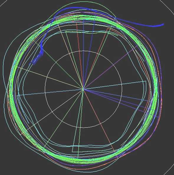
Graph 2. Plan view of the trajectories of the particles.
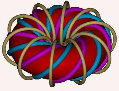
Graph 1 . View of the modelled stellarator
Graph 2. Plan view of the trajectories of the particles.
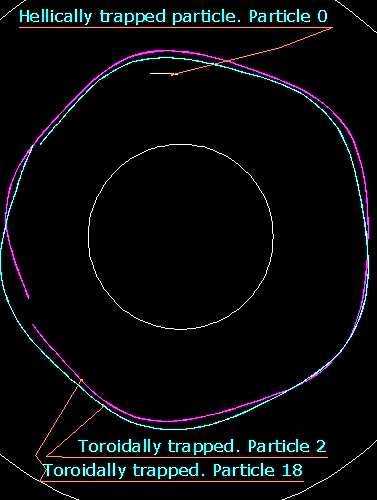
Graph 3 . Trajectories of 3 trapped particles. Plan view.
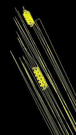
Graph 4 . Detail of the poloidal view of the hellically trapped particle number 0
Last Update 26-10-2005