Abstract :
A new module of SimPIMF is improved and tested. The new
version is named SimPIMF v1.2 . The drift velocities are removed and a
double approximation over the field lines is introduced. The effect of the
step time and the size of the magnetic grid on the resulting magnetic
surfaces is tested. new module of SimPIMF is improved and tested.
General description
The module is an
evolution of the code described in [1] and [2] where the part for the
simulation of magnetic surfaces has been separated from the part to follow
magnetic field lines. So the speed to calculate magnetic surfaces has
increased more than 10 times.
The present code is denoted as SimPIMF v1.2
It also calculates the rotational transform by computing the toroidal and
poloidal revolutions for each particle.
Modelling
The vacuum magnetic field is obtained using
MEMCEI v2.1 code [4]. The model is a classical stellarator with l=2 m=6 that
have similar dimensions to CTH, a l=2 m=5 torsatron in Auburn University.
The model is shown in Graph 1.
In this calculation the currents are the same as in [1]
From 1 to 10 Msteps of step time 10 and 100 picoseconds and Te=1keV are used.
It depends on the necessary accuracy or the type of test for the code.
Three magnetic grids are tested,
Grid A : with 21 x 21 x 9 nodes = 3969 nodes
Grid B : 41 x 41 x 17 nodes = 28577 nodes
Grid C : A finest grid with 61 x 61 x 25 nodes = 93025 nodes .
The objective is to know up to what degree the inaccuracies of the magnetic
field grid affects the calculated magnetic surfaces.
Some results
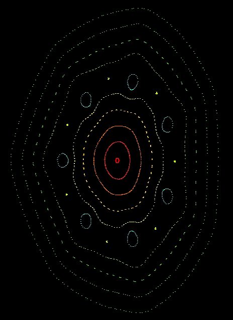
The result in Graph 2 was obtained under the next conditions: Grid A , 7Msteps in most of the graph, step time 10 pisosec. , 22 particles that born at different radial positions with increase of 2,25mm, particles starts from the plane y=0.
Some other surfaces are added to the 22 obtained before. Since most of the rational surfaces do not never pass through the point of birth of particles, only some magnetic islands appear in the first run of the code. The other magnetic islands are obtained manually by throwing a particle from an adequate place, in general near the centre of a region with lack of field lines. In general 10MSteps are used for the islands.
The rotational transform at the second surface in the Graph 2 is Iota = 0,2866 and at the island in the “stochastic” region is 1/3.
The external region should be a stochastic region similar to the one in W7-X [5] because the external points in yellow corresponds to one particle which travels all around nearly randomly.
In contrast the 3 magnetic islands in dark pink near the perimeter are clearly confined in its regions. For example the tree regions in dark pink are independent (one only particle cannot generate the 6 islands) of the 3 symmetrical islands in magenta. Note: The respective dark pink islands in the other group of 3 islands has not been generated.
If one particle is thrown at slightly higher radial position the particle is lost after a few turns.
Analysis of islands
Apart from higher order, the main islands observed in Graph 2 are:
(The values expressed below are : calculated iota, supposed instability mode, some decimals of the rational)
Iota = 0.3359 ~=1/3 : Two groups of 3 islands at the border
Iota = 0.30748 ~=4/13 = 0.3077... : 13 islands in light blue
Iota = 0.2981 ~= 3/10 : 2 groups of 10 islands in olive green
In Graph 3, which is a new calculation of only the central part of the Graph 1, islands :
Iota = 0.2817 ~= 2/7 = 0.2857... : 7 islands near the centre, colour cyan.
These rationals are the only important rationals up to n=6 (Iota = n/m). This can be observed in [3].
More accurate grids
The same process described above is done with the Grid B and the result is shown in Graph 4 . In this case only the bigger islands appear clearly. It seems that the field errors due to the grid effect have been reduced.
The width of the 1/3 island in Grid A is roughly = 25mm. In Grid B it is approximately 17mm.
This might follow the expression W = width of islands = ( Berrors / S)0.5 , Berrors = resonating magnetic field errors , S = magnetic shear [4].
Ratio of BerrorsB = WA2 / WB2 = 2.16 (using Wa=25 and Wb=17mm), similar to the ratio of grid lineal elements.
The other islands are very small or have disappeared.
Graph 5 shows a calculation with the Grid C . Smaller 1/3 islands can be seen here. The magnetic surfaces are slightly more perfect than in Graph 4.
Graph 4 and 5 are obtained under the conditions: 1Mstep, step time 0.1 nanosec. , 22 particles that born at different radial positions with increase of 2.25mm, particles starts from the plane y=0. In Graph 5 three external particles are added (reddish colours). The generation took 45 min.
Conclusion
At least a grid of the type B has to be used when calculating magnetic surfaces for any coil configuration. The processing time is consumed only during the calculation of the grid so it does not influence on the simulation time. Only more memory is required but no a limiting issue.
Further developments
Some configurations of deformed or misaligned coils will be calculated. It will further test the code and additionally establish the maximum coil errors to have acceptable magnetic surfaces.
References
[1] "Simulation of magnetic surfaces in a classical stellarator using SimPIMF v1.0", Vicente M. Queral . See “Past research"
[2] "Simulation of trapped particles for the optimization of UST_1 coils", Vicente M. Queral . See “Past research"
[3] "Optimum Iota Profiles", Vicente M. Queral . See “Past research"
[4] "STELLARATORS" , D.A. Hartmann, Max-Planck Institut für Plasmaphysik.
[5] "Physics and engineering design for wendelstein 7-X" Craig Beidler, et al. Fusion Tech. 1989

Graph 2 . Magnetic surfaces in the studied stellarator at toroidal 0º . Real width of the picture 175mm
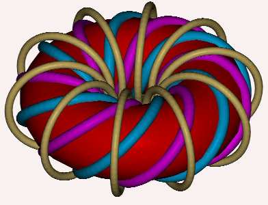
Graph 1 . View of the modelled stellarator
Graph 2 . Magnetic surfaces in the studied stellarator at toroidal 0º . Real width of the picture 175mm
Graph 3 . Magnetic surfaces and magnetic islands from the simulation of the central area, at toroidal 0º . Real width of the picture 16mm
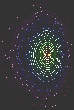
Graph 4 . Magnetic surfaces related to the Grid B at toroidal 0º
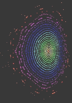
Graph 5 . Magnetic surfaces related to the Grid C at toroidal 0º
Last Update 10-11-2005