Abstract : Simulations of the standard configuration in HSX 'Helically Symmetric Experiment' are carried out and compared with simulations in UST_1-large. Results are compared with the ones from HSX team in order to further validate SimPIMF code. Iota profile, ripple, magnetic surfaces, drift orbits and trapped particles are simulated for HSX and UST_1 and compared. The results from SimPIMF agree notable well with the results from HSX team.
HSX, Helically Symmetric Experiment, in University of Wisconsin-Madison, USA, is a stellarator focussed in the study and improvement of neoclassical transport. Features : major radius = 1.2m , minor radius = 0.15m, plasma volume = 0.44m3 , magnetic field = 0.5T , rotational transform = 1.05 to 1.12 , 4 periods and 48 coils, [1].
Objectives :
* Further test SimPIMF code. If results from HSX team and from SimPIMF are similar it further validates the code.
* Better understand HSX style stellarators. Quasi-symmetric and in particular quasi-helical stellarators.
* Only an abstract of the results and simulations are shown. Few figures are presented now due to lack of time to publish them..
Modellisation
UST_1 is scaled by a factor of 8 to obtain a size similar to the size of HSX. The major radius is smaller in UST_1 and the minor radius larger because UST_1 is relatively compact (Aspect ratio = 6) and HSX has large aspect ratio.
The name of the UST_1 stellarator scaled 8 times is "UST_1_Size-HSX" in the present page.
Presently the code allows changing from one model to another in few seconds. Four models are available: CNT stellarator, HSX, UST_1 and UST_1_Size-HSX.
HSX is modelled using the multifilamentary structure of coils kindly supplied by the HSX team. Each coil is defined by 842 segments that form 16 turns. In total 40416 segments.
A new module to save MagneticGrid structures is created in SimPIMF to obtain the values of B from a file. Otherwise the calculation of the Grid is too slow for such a high number of segments. The module to load MagneticGrid files was already available.
UST_1_Size-HSX is created like in UST_1 but incluiding a scaling factor of 8.
B on axis is set to 0.5T in UST_1_Size-HSX.
Currents
* In HSX : current TF = 5361 A (model of 16 turns per coil and 48 coils)
* In UST_1_Size-HSX : current TF = 220000 A (model with 1 turn per coil and 12 coils)
* Magnetic field on axis for UST_1_Size-HSX has a maximum of 0.54T and a minimum of 0.488T.
* Magnetic field on axis for HSX is very similar to 0.5T at any point on the axis. Minimum 0.499 , maximum 0.504T. Ripple on axis is practically null.
Magnetic axis
The simulation of HSX with simPIMF gives the magnetic axis exactly on x=1.4454m (at toroidal = 0º). It is the value povided by the HSX team. The axis obtained from the simulation is notable helical.
Magnetic axis in UST_1_Size-HSX appears at x=1.0052m. Minor radius = 0.168m.
Ripple
Maximums and minimums of |B| have the same value and they are uniformly distributed . It is a key feature in HSX. See Fig. 1.
Ripple in HSX is null on axis and low in general. Small secondary ripple, probably modular ripple, is observed.
Ripple in UST_1 is high and the stellarator is not quasi-symmetric. See [2] for further information and graphs. Large modular ripple (only 12 coils) appears in UST_1.
Magnetic surfaces in HSX
Magnetic surfaces are simulated and represented by SimPIMF code for the conditions :
130 particles are thrown. 1mm between them. It is the fine simulation. Other simulations are carried out but not shown.
Coef MagneticGrid = 20 = 1/20m between nodes.
Poincare simulation, without drifts.
The result is shown in Fig 2.
Fig. 2 is similar to the one from HSX team but the small differences are not analysed here. The comparison of drift orbits in UST_1 and HSX is the most important task in this page.
Iota profile in HSX
Conditions of the simulation :.
- Calculation with drift and electrons of energy = 50eV. It is a value cited in [5] but it is not clear if 20eV or 50eV is the correct value. In any case the difference is small.
- 60 points of data.
The accurate result (around 1200 turns of the electron) is very similar to the less accurate one (about 200 turns).
Results :
The graph is shwon in Fig 3.
Comments :
- The result is similar to the theoretical one from HSX team [5] Fig 1. The error is less than +-0.01. This further validates SimPIMF code.
- There is a strange behaviour near r/a=1 that usually is caused by islands. Not analysed now.
- Points near the axis cannot be calculated by the code but the number of rejected points is high in HSX perhaps due to the large excursion of the magnetic axis.
Rationals and islands
They are not studied in HSX. They were studied in UST_1 and CNT stellarators.
Major islands are not observed in Fig 2.
Drift orbits in Boozer-like coordinates
in HSX and UST_1
HSX
[1], slide "Trapped Particle Orbits", presents the results of a simulation of a 25KeV electron thrown at pitch angle of 80º. The particle remains approximately on the magnetic surface and does not escape.
SimPIMF simulation in HSX
80º corresponds to Vt=0.1736 in SimPIMF (the relative tangential component).
Conditions of the simulation :
Energy of the electron = 25keV
Vt=0.1736
Simulation with drifts, collisionless regime.
Point of birth of the particle : On Y=0 plane , z = -0.1m
Results :
The electron does not escape with SimPIMF code either. This further supports the correction of SimPIMF for more complex simulations.
Fig. 5 shows the result of the representation in Boozer-like coordinates for a relatively long period of time, 100 microsec.
The electron executes a thin and short banana orbit around the magnetic surface, in magenta, together with a toroidal precession movement. The electron turns poloidally and seems able to pass from one helical period to another in collisionless regime. This behaviour seems the correct according to [1] and it is extraordinary in comparison to UST_1 and any other present stellarator.
In red the representation of a sequence of points of the orbit in Boozer-like coordinates during the 100 microseconds of simulation. The electron does not escape and it remains near the magnetic surface (in yellow).
Questions :
* Is the behaviour of the electron the same under any condition? (energy, pitch angle, birth point)
* Is the behaviour of a proton similar?. For W7-X, in [3], it is stated : "For neoclassical ion transport, configurational details are less important than the presence of a radial electric field, which.... reduces the diffusion coefficient well below the plateau regime. Therefore, electron behaviour is of great importance since it is less affected by the electric field (electrons largely being in the 1/nu regime)". So, will the protons-ions escape as fast as in UST_1 or will the confinement of ions be improved due to quasi-symmetry?
* How are the magnetic surfaces defined in relation to the drift velocity to keep the particles confined?. Very possibly HSX has been calculated using a NESCOIL-like code and the process is inverse. In spite of this the question is important.
UST_1 large size (UST_1_Size-HSX)
Conditions of the simulation
Energy of the electron = 25keV
Vt=0.3 (otherwise it is a modular ripple trapped electron . ~12 coils only)
Drifts simulation, collisionless regime
Point of birth of the particle : ( 0, 0.9808 , 0.0768) . It is a minimum, a correct point to obtain a helically trapped particle.
Results
Fig. 6 shows the drift orbit of the trapped electron. It is a direct lost. A similar result was obtained for UST_1 (real size) in [4].
Drift speed is 54291 m/s from SimpIMF and 55932 from an approximate analytical calculation. So the electron escapes roughly in 3 microsec.
Drift speed from simulation is 29557 m/s in HSX (smaller, partly because HSX is less compact than UST_1). But drifts are compensated along the orbit in HSX.
Possible future research
Simulate protons or D at high energy in HSX. Detailed simulation of the drift orbit along a small distance. Comparison of neoclassical flux of particles in UST_1 and HSX.
Acknowledgments
I thank the HSX team because they kindly provided the definition of HSX coils and other necessary information to simulate HSX.
References
[1] "Comparison of Electron Cyclotron Heating Results in the Helically Symmetric Experiment with and without quasi-symmetry" K.M.Likin On behalf of HSX Team , 30th EPS conference, St. Petersburg, Russia, July, 7-11, 2003
[2] "Simulations in UST_1. Magnetic surfaces, islands, Iota and Magnetic Well profiles" , Vicente M. Queral. See List of all R&D
[3] "Physics and engineering design for wendelstein 7-X" Craig Beidler, G. Grieger , et al. Fusion Tech. 1989
[4] "Toroidal, helical and modular ripple trapped particles in UST_1. Representation in Boozer-like coordinates" Vicente M. Queral. See List of all R&D .
[5] "Drift Orbit and Magnetic
Surface Measurements in the Helically Symmetric Experiment" J.N. Talmadge,
V. Sakaguchi et al.
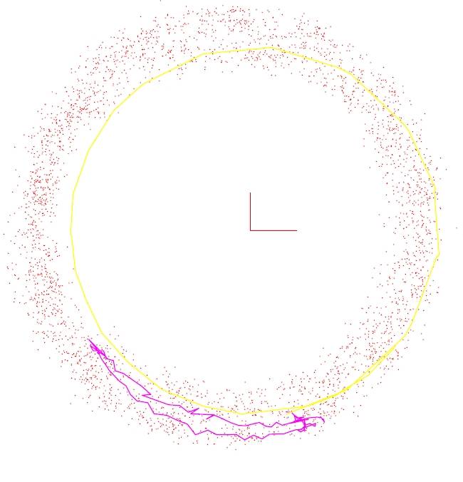
Fig. 5 . Simulations in HSX in Boozer-like coordinates. In magenta a banana orbit for the conditions of the simulation (electron 25keV ...). In yellow the passing orbit without drifts. Red points are the successive points belonging to the drift orbit which is a sequence of bananas, for 100 microseconds. The points always remain near the passing orbit. The confinement of electrons is excellent even for this extremely high energy (for a size and B like in HSX). In UST_1 they escape after ~3 microseconds. The magenta banana appears poorly defined because this thin banana is at the limit of the resolution of the Boozer-like method in SimPIMF.

Fig. 1 . B on x=magnetic axis + 50mm in HSX . Graph comes from SimPIMF. Maximums and minimums of |B| have the same value and they are uniformly spaced.
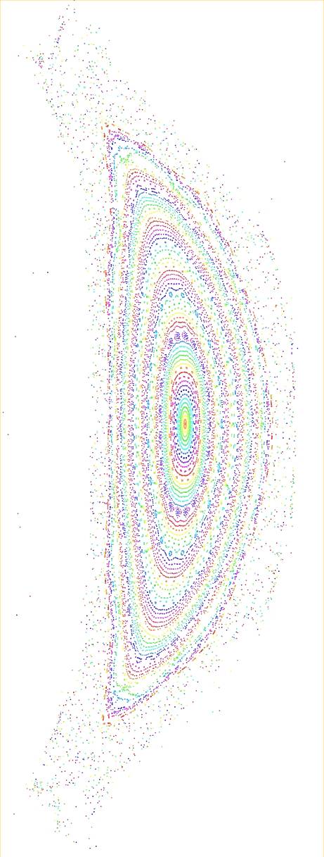
Fig 2 . Magnetic surfaces simulated with SimPIMF. It is the accurate simulation : 130 surfaces, 1mm between them. Simulation without drifts.
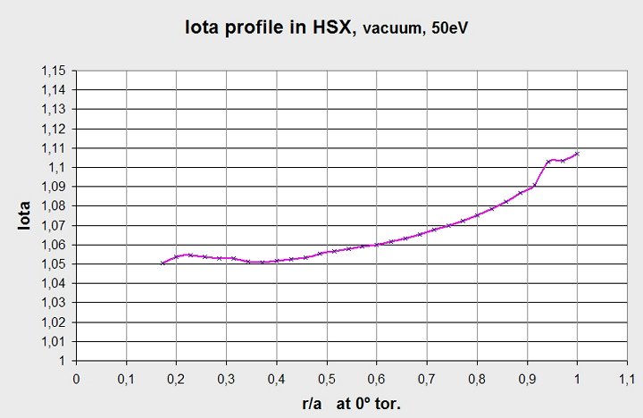
Fig 3 . Iota profile in HSX calculated by SimPIMF. Deviations smaller than +-0.01 are observed in the value of Iota
Fig. 5 . Simulations in HSX in Boozer-like coordinates. In magenta a banana orbit for the conditions of the simulation (electron 25keV ...). In yellow the passing orbit without drifs. Red points are the sucesive points belonging to the drif orbit which is a sequence of bananas, for 100 microseconds. The points always remain near the passing orbit. The confinement of electrons is excellent even for this extremely high energy (for a size and B like in HSX). In UST_1 they scape after. The magenta banana appears poorly defined because this thin banana is at the limit of the resolution of the Boozer-like method in SimPIMF.

Fig 6 . In
Magenta trajectory of a helically trapped electron in Boozer-like
coordinates for an UST_1-scaled stellarator of size similar to HSX. The
conditions of the simulation are 25keV and other (read text).
In yellow the orbit
of an electron simulated without drifts (passing orbit) thrown from the same
point
Date of publication 28-01-2007